Consider the problem of intervening on the behavior of a language model, say to make it less gender biased when processing the word developer, or nurse. If one identifies activations in the network that cause a biased prediction, one might intervene to change those activations. But one has no guarantees how that intervention would affect the network in other contexts, say for other prefixes of text. In this blog post, we’ll detail the Backpack, a new neural architecture that allows for interventions on non-contextual word2vec-like word embeddings that have global, predictable effects on the log-predictions of the language model, for any prefix.
The Backpack is a drop-in replacement for the Transformer that provides new tools for interpretability-through-control while still enabling strong language models.
- We’ll discuss the design motivation for Backpacks and what distinguishes them from Transformers, RNNs, and most other sequence architectures.
- We’ll demonstrate examples of how we’ve used the Backpack structure to implement precise interventions.
- Then, we’ll walk through the code, discussing details and showing how easy it is to implement.
Monolithic functions and control
Neural sequence modeling usually proceeds by computing non-linear featurizations of each prefix in a single monolithic function, and modeling distributions over sequences through the product of distributions over “next token” given “context”.
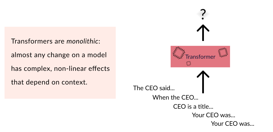
By monolithic, we mean that all features for all words are non-linearly combined and there is (effectively) no guarantee on the functional form computed. For almost all internal activations of, e.g., Transformers and RNNs, any change to the input can have unpredictable effects on the activations’ values.
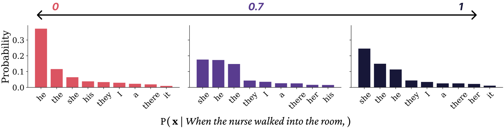
To make this concrete, consider a gender bias issue that’s prevalent in neural LMs: certain stereotypically gendered career nouns lead to highly biased distributions over pronouns (like he/she/they). For example, for the prefix The CEO said, one can observe that LMs tend to place much more probability on he than she:
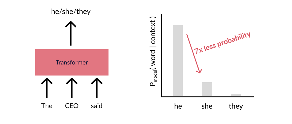
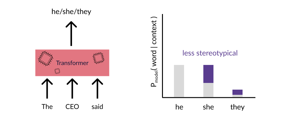
One might try a clever patch to the model, changing some activations, performing fine-tuning, etc. One can then check that the probabilities change as desired:
The trick with monolithic functions in language, however, is that there’s a combinatorially large space of inputs, and no guarantees on how the different prefixes will change how the patch or intervention or finetuning or RLHF affects all combinatorially many possible contexts. Everything from in-context learning to prompt hacking shows the difficulty of knowing how different prompts will affect the contextual behavior of a network. It’s a toy example, but consider if we just changed the prefix to The CEO thought. Do we have any guarantee that the intervention we made to fix the “CEO” problem will have the same effect in this context?
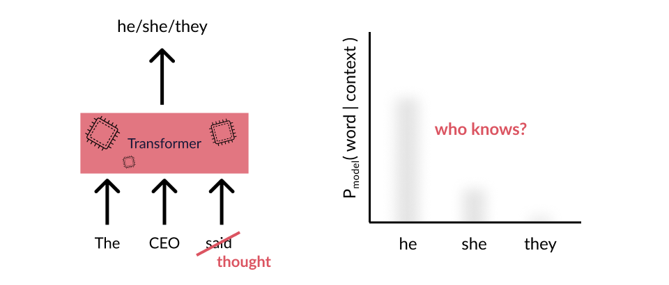
Likely not; all contextual activations of the network could vary in (effectively) arbitrary ways. Maybe things will go well, but we can’t tell before trying each possibility…
The Backpack is intended to fill a gap in the zoo of neural architectures in which one needs expressivity akin to a Transformer, but still wants to be able to perform a set of reliable interventions whose meanings are predictable regardless of context. We’ll find that our trained models learn rich, non-contextual semantics that one can intervene on.
The Backpack Language Model
Backpack models operate on sequences, and differ from most neural models in that their outputs are exclusively the result of a weighted sum of non-contextual feature represenations of individual input symbols. These non-contextual features are dynamically weighted (by a context-dependent function) between 0 and 1, and summed, to make the final (log-)prediction of the model.
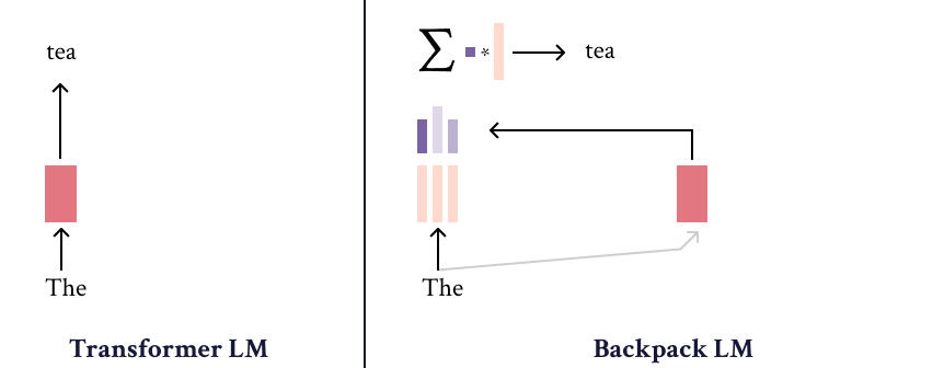
As such, Backpacks operate in two steps. The first is to produce sense vectors for each symbol in the input. The sense vectors intuitively represent the different ways in which the symbol can be predictively useful in different contexts. A bit formally, let \(\mathcal{V}\) be a finite vocabulary (like of subwords of a neural LM.) Then for each word \(x\in\mathcal{V}\) in the vocabulary, \(k\) (a hyperparameter) sense vectors are defined:
\[c(x)_\ell \in \mathbb{R}^d, \ \ \ \ \ell\in\{1,\dots,k\}\]When we go through the code, we’ll talk about how these vectors are parameterized. But each is a vector in \(\mathbb{R}^d\), the dimensionality of the hidden states of the model.
Given a sequence \(x_1,\dots,x_n\), we take the sense vectors for all the words in the sequence:
\[c(x_1),\dots,c(x_n)\]which when represented as a tensor is in the space \(\mathbb{R}^{n\times k \times d}\); there are \(n\) elements of the sequence, each with \(k\) senses, and each sense of dimensionality \(d\).
To compute the contextual representation of a symbol, \(o_i\in\mathbb{R}^d\) that represents \(x_i\) in the context of the prefix \(x_{<i}\), the senses of all words in the prefix are weighted by a non-negative factor, and summed:
\[o_i = \sum_{j=1}^{i} \sum_{\ell=1}^k \alpha_{ij\ell} c(x_j)_\ell\]
The expressivity of the network comes largely from the contextual computation of the summation weights \(\alpha\in\mathbb{R}^{n\times n\times k}\). In fact, in all of our experiments, we use an entire Transformer stack just to compute the averaging weights. We’ll go into more detail as we go over the code, or feel free to check out our paper for the mathematical details.
That’s effectively the whole model. For Backpack Language Models, we simply take the \(o_i\) representation and linearly transform to the space \(\mathcal{V}\) and take the softmax to predict the next word:
\[x_i \mid x_{<i} \sim \text{softmax}\left(Eo_{i-1}\right)\]where \(E\in\mathbb{R}^{\vert\mathcal{V}\vert\times d}\).
Emergent structure in sense vectors
We’re now going to visualize some of the sense vectors learned by Backpack Language Models. For example, we’ll take a sense vector like \(c(\text{science})_3\), the third sense vector of the word science, and visualize it by multiplying it by the softmax matrix, \(Ec(\text{science})_3\), and sorting to see the highest-scoring and lowest-scoring words.
Before we look, I’ll go into why this visualization makes sense. Looking at our probabilistic model above, the log-probabilities of next-word-given-prefix are \(Eo_{i-1}\). The \(o_{i-1}\) representation is just a non-negative weighted sum of sense vectors, so whenever the word science is in a prefix, say at index \(j\), it contributes to predicting future word \(i\) via the term
\[\alpha_{ij3} E c(\text{science})_3 \in \mathbb{R}^{\vert\mathcal{V}\vert}.\]The \(\alpha\) is a term between \(0\) and \(1\), so the direction \(Ec(\text{science})_3\) is unchanged; hence, the contribution direction of this sense vector to the log-probabilities is exactly what we’ll visualize.
Here are some of the top-scoring words for different senses of the word science, and some intuitive categories we’ve labelled for them.
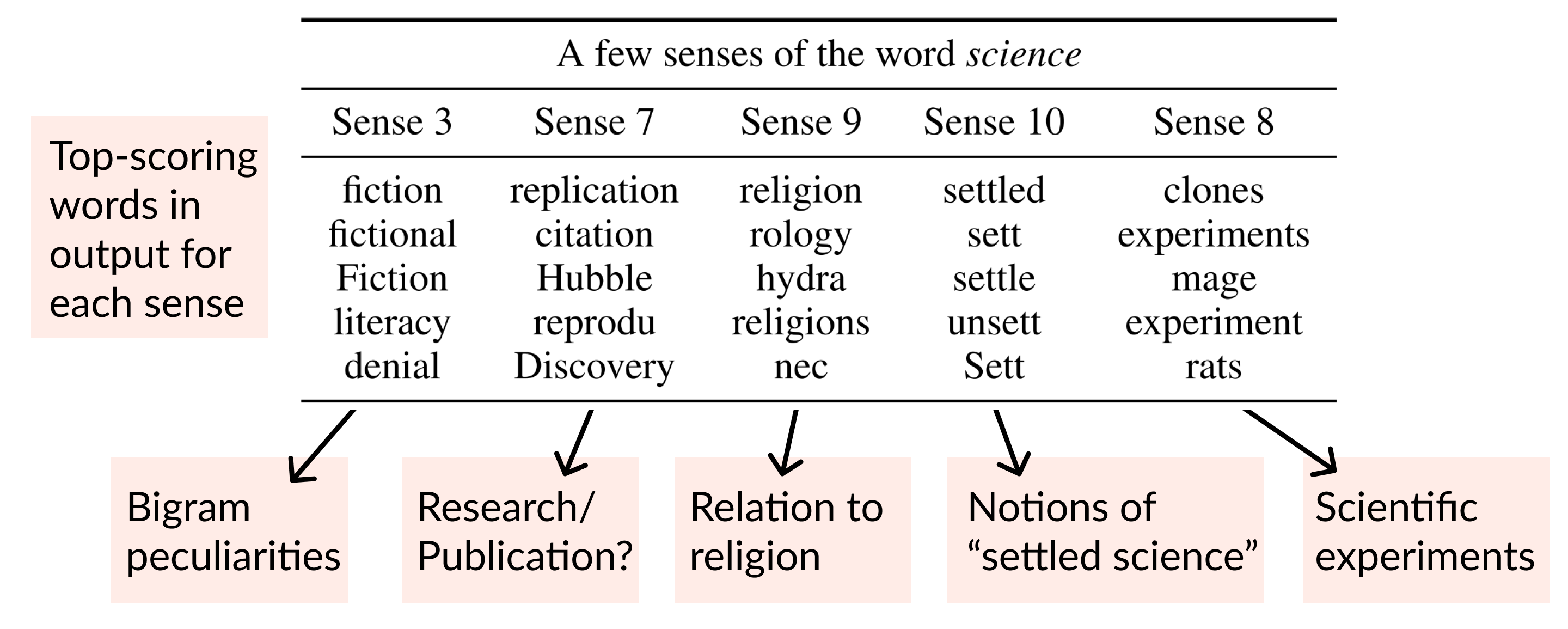
Not all senses have such coherent categories, but they seem to richly decompose the potential predictive contributions of a word.
Some sense indices seem to have consistent meanings, at least for large classes of words.
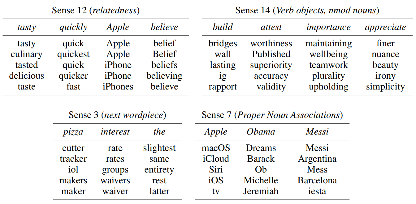
You can explore sense vectors yourself through our demo.
The main takeaway of sense vector emergent structure is that, due to specialization and consistent meaning in all contexts, the senses may make good targets for intervention.
Examples of Control
Code Walkthrough
Here, we give an overview of the crucial components of the Backpack in pseudocode. We use a slightly simplified version compared to our released models.
The Backpack
The Backpack proceeds in a few parts. First, we get senses of each word in the context
senses = sense_network(input_ids) # (bs, nv, s, d)
Next, we also get contextualized hidden states for all prefixes via a Transformer:
hidden_states = transformer(input_ids) # (bs, nv, d)
From the hidden states, we compute pairwise contextualization weights for all senses via multi-head self-attention-like weight computation (without value averaging)
contextualization_weights = self_attention(hidden_states, values=False) # (bs, nv, s, s)
Now, we just perform the averaging and sum over senses to get the backpack representation:
outputs = contextualization @ senses # (bs, nv, s, d)
outputs = outputs.sum(dim=1) # (bs, s, d)
Now we’ll go into a bit of detail for sense_network.
Sense Network
To construct sense vectors, we embed each word, and then pass through a feed-forward network
mlp = MLP(
  input_dim=d_model,
  intermediate_dim=5*d_model,
  output_dim=num_senses*d_model
)

# Embed words
embeds = word_embedding(input_ids) # no position embeddings

# Map to higher-dim space via MLP
senses = mlp(input_ids) # (batchsize, seqlen, num_senses*d_model)

# Reshape to get num_senses vectors
senses = senses.reshape(batchsize, seqlen, num_senses, d_model)
We share the word embeddings with the underlying Transformer.
Citation
@InProceedings{hewitt2023backpack,
  author =      "Hewitt, John and Thickstun, John and Manning, Christopher D. and Liang, Percy",
  title =       "Backpack Language Models",
  booktitle =   "Proceedings of the Association for Computational Linguistics",
  year =        "2023",
  publisher =   "Association for Computational Linguistics",
  location =    "Toronto, Canada",
}